Automata Sandbox Simulation
Carlos Ramos
- Link to the repo: https://github.com/0x7b1/cellular-automata-fluid-simulation
- Executable: http://kodu.ut.ee/~jramos/public/executables.zip
This project will implement a sandbox simulation of liquid physics using cellular automata. The simulation will invite users to explore their creativity and think about ways to create different scenarios and see the reactions with objects by being able to make modifications in real time. To achieve the dynamics of fluid, this project will implement different sets of cellular automata rules and formulas needed for the physical constraints. This program will be implemented for the desktop in order to get the most out of the computer resources using a low level language. (compared to the web or mobile).
Background and Motivation
There exists a kind of simulation called “Falling-sand” which are games that provide a canvas to paint different elements and see how the particles interact between them in different ways. These games have been around for a while allowing you to interact with different mechanics and using creative elements. Some of them achieve really complex element behaviors and others are actually implementations of academic research. To mention just a few we have The Powder Toy, dan-ball.jp’s Powder Game as the oldest ones, and Sandspiel and Noita which are very recent games implemented with new approaches/techniques.

The Powder Toy
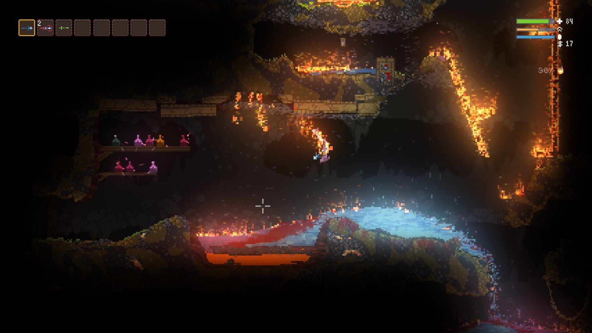
Noita
What they have in common is the use of cellular automata to make the elements interact with each other which are based on rules that have an evolving nature. Simulation of fluid physics is hard to implement and there are multiple approaches for doing it. Although the use of Navier–Stokes equations can achieve good results, cellular automata provides an interesting, appealing, and cheaper way to get similar results. The goal of the project is to provide the ability to interact with the sandbox in real time with the provided tools (that will be described above). Furthermore, this simulation is a low-res 2D grid based style. To do so, many things have to be taken into consideration such as the implementation of the algorithm, the environment and development tooling, and a good sense of mathematics. These are the main motivations for doing this project.
Being described what the project is about, now the description of features are going to be presented.
- Spawn liquid: This is the main feature because it will allow the user to create chunks of liquid from the mouse position within the canvas. This portion of liquid will immediately start to interact with the other elements wherever it is being placed.
- Create solid walls: This feature will allow liquid to collide with solid objects that can be painted with the mouse. The option for erasing wall pixels is also considered.
- Rotate canvas: This is a personal challenging feature. With this the user has the ability to grab the canvas and rotate (around the mass center of the canvas) in XY direction and see how the liquid reacts with the solid objects and gravity.
Resources
As was introduced before, this program will be implemented for the desktop in a low level language, namely Rust to achieve cross-compatibility and stable performance. Although it is true that it is feasible to port to the web, it is not a short-term priority.
Goals and Deliverables
The final goal of the course project is to deliver the program described above. It might have some modifications in the process but they must not be something different to the planned. Also, the final result may not result visually appealing but the underlying research and implementation should be solid. If the project turns out to be very complex and it is taking time, the feature to be sacrificed will be the third one “Rotate canvas”. Now a rough list of tasks and subtask will be described in order to be executed within a semester which encompasses 6 milestones.
Tasks
- Set up the interactive canvas in Rust
- Implement a basic CA
- Write out the progress, research, results
- Implement the liquid simulation
- Try different scenarios
- Implement liquid coloring
- Implement collision with solids
- Implement gravitation in canvas rotation
- Implement the visual UI (texts, buttons)
- Implement the painting/placing of solid pixels
- Implement the erase feature to remove solid pixels
- Implement the canvas rotation
- Test different scenarios
- Implement liquid shading
- Code profiling and optimizations
Tracking
I am going to use Clickup for keeping track of the real tasks of the milestones. This tool is a handy option for showing the progress, including planned time, tracked time, and status, with my own workflow without having to write them once again in this wiki.
Milestone 1 (06 March)
For this initial milestone the list of tasks were more focused on the beginning stage of the project. They will be listed and be explained on what have been achieved.
- Brush up the practice on Rust
- Play around with some stable and flexible graphics API
- Setup simulation structures, canvas and code
- Implement a basic CA
Brush up the practice on Rust
Initially this language was decided to be used because it provides many benefits related to performance. However its relatively steep learning curve required it to dedicate a decent amount of time trying to learn the features and quirks of the language to start doing the main work. As my experience goes, I had some experience with Rust a while ago but I didn’t dig properly into its fascinating and well-known features that make it unique. That was my goal for this task, to try to re learn the language and practice to gain more experience by using the language enough with the concepts that would make the simulation be fast and secure. The main resources utilized now and throughout the progress of this project are:
Play around with some stable and flexible graphics API
The road to pick the desired graphics library involved to try and implement fair enough code and decide which one to choose. The starting point was this resource which gives a great insight on which kind of library to use. By popularity, the most used starred in Rust is named gfx which leverages the power of Vulkan in the Desktop. However, as the complexity of using low level APIs is out of scope of this project, these kinds of libraries were discarded (as well as those one who are wrappers of OpenGL, DirectX). Later I found two promising 2D graphics libraries which provide good constructs, methods and structs to work with, those are graphics and minifb. These are not quite popular but suits the needs of this project. After experimenting with both, the picked one was the latter because the handling of input events, buffer allocation and pixel rendering were more convenient (also because it provides a nice math library for doing color and vec operations).

Trivial implementation of noise pixel rendering using minifb.
Setup simulation structures, canvas and code
After trying to visualize the whole picture of structures needed for the simulation, the tentative ones to be used (for now) are: Cell and World. Cell holds the properties of a single pixel in the grid; World holds the grid which is a matrix of Cells. Each one has its own methods to handle and update the data. Cell contains methods for updating its internal state (coloring), and World does the respective manipulations of cell evolution (creating a new generation) of cells. The purpose of this task was also to gain familiarity with Rust features such as traits, structs, I/O streams and boxes (memory heap allocations).
Implement a basic CA
To tackle this task with the purpose of revealing the power of the graphics library in conjunction with the features of this programming language, a basic Cellular Automata (CA) rule was implemented, namely, The Conway’s Game of Life. The Game of Life is a simulation which models the life cycle of bacteria using a 2D cell grid. Given an initial pattern, the simulation runs the birth and death of future generations of cells using a simple set of rules. CA is a model of a system of cell objects with the characteristics of living in a grid, having a single state, and being aware of the neighbors. For now just imagine having a grid being occupied by a single living cell, now at each iteration the following set of rules will be applied to the neighbors of a cell.
- A location that has zero or one neighbors will be empty in the next generation. If a cell was there, it dies.
- A location with two neighbors is stable. If it had a cell, it still contains a cell. If it was empty, it's still empty.
- A location with three neighbors will contain a cell in the next generation. If it was unoccupied before, a new cell is born. If it currently contains a cell, the cell remains.
- A location with four or more neighbors will be empty in the next generation. If there was a cell in that location, it would die of overcrowding.

Neighbors of a cell (courtesy of natureofcode.com)
And that’s it, the final result of this task shows how the implementation runs for Conway's simulation and reveals the bacteria growing over time.

The Game of Life in execution
For the next milestone the tasks will be focused on improving the inner implementation of the cellular automata to make it more flexible to the distinct types of elements that the simulation will handle in the future (water). Also to implement the paint feature of solid elements in the canvas.
Milestone 2 (20 March)
For this stage the task were focused on:
- Improving the implementation of the cellular automata to make it more flexible for further elements and logic
- Implement the brush feature of solid cells in the canvas
Improving the implementation
So far the experience with Rust has been delightful but also a bit painful. There have been some concepts that needed to take time and practice, this is memory handling. Rust is not as permissive as other languages when it comes to memory errors. Usually all the work has to be done upfront. This means that all the handling of null variables, undefined states or memory corruption is checked at compile time. In general I’m getting used to this kind of programming because it helps a lot when dealing with huge amounts of instances that are supposed to be unpredictable and change over time. To this extent the code has been improved as I could. I’m not implementing my own cargo libraries yet but soon I will because code modularization is becoming a need.
Implement the brush feature of solid cells
For this part I decided to make some changes in the draw logic of the simulation. First, I got rid of the initial implementation which started a new simulation based on a file which described the initial state of the cell world. Now it starts with a blank canvas to start drawing. The drawing part is made of mouse clicking and dragging. Internally does not draw every single trace in which the mouse has been located. Instead is updated on a fixed interval and it draws a fixed size of pixels on the mouse location. Two sizes of brushes were implemented, a small one and a big.

Two sizes of brush
But as you may notice this is not being animated, because it should be like that. This brush is a solid element which has to collide with the water in the future. However I also wanted to have my early simulation working with this. So, how do I evolve the cells in the canvas taking into consideration the new constains? I decided to implement that task for the next milestone. For now I just got fun and implemented the drawing feature with different types of brushes ,or may say, different types of CAs (the most interesting ones). Also the animation can be paused to have the opportunity to draw and see how this evolves without any evolution and then simulate again. That’s it for now. I have been also implementing coloring and multithreading but it’s buggy for now.

CA shapes as brush type
For the next milestone I plan to implement the logic of CA animation with gravity, which also has to respect the solid objects constraints. Coloring of elements as well and some further improvement in the performance.
Milestone 3 (03 Apr)
For this milestone the achieved tasks are:
- Implementation/experimentation of the CA rule for gravity and water fluid simulation.
- Coloring of elements
Implementation of fluid dynamics
At first, before choosing this project idea in the first place I had a vague idea of how exactly I should implement the behaviour of water in a Cellular Automata fashion. Now, after devoting a decent amount of time doing research in the topic I’ve found different strategies to tackle the problem. I’ve implemented two of them.
1-Dimensional CA
This method is based on this post in which the simulation is made using a single dimension of cell interaction. Each cell in the vector has 3 values: elevation, water, volume and kinetic energy Then the simulation works with the values generated by those inputs: potential energy and directional pressures. In every iteration, each cell calculates the amount of pressure with their neighbors and the difference between them and itself. Later, each cell finds a value used to determine the amount of water going to the next direction. These values are added at the end of the iteration. The implementation required to tweak the initial implementation quite a lot since it required downgrade the dimensionality of the cell space. The result I got was not compelling, as it required more time to fix and debug. I decided to try another approach instead.

1D CA Fluid simulation
2-Dimensional CA
Using two-dimensional space of cells to represent the world was the way to go. Each cell can contain different elements and interact with others. The algorithm is heavily inspired by the Chapter 2.6 of the book Game Programming Gems Series v. 3. The basic idea is to start by considering two or more water cells stacked vertically. When this occurs, then the cell of the bottoms starts to get more water level than the others. This way we avoid tracking expensive calculations of pressure to make water equalize. We only get the current value level of the water and move it upwards when is stacked up. The list of constants used for the simulation are: flow, mass, speed. The algorithm requires that if one cell contains 1.0 units of water, the cell below it should contain up to 1.02 units, the next one 1.04, and so on by a factor of 0.02. There is a special case to get the simulation run fluid. The bottom cell has to contain a proportionally smaller excess amount of water and compression than the others. The water movement is made by evolving the generation of cells of the mass matrix with the following rules:
- Get how much water the bottom cell should contain using the mass of the current cell and the cell below. If is below 0 (or the threshold), remove the corresponding amount from the current cell and add to the bottom cell
- Update the cell to the left. If it has less water, move over enough water to make both cells contain the same amount.
- Repeat the process for the right cell
- Same procedure as step 1 but with the upper cell.
It is required to keep track of the current water values on each generation to be updated in the next one The computation is a bit expensive but provides a better looking simulation.

2D CA Fluid simulation
The author of the book suggests many other elements (fire, heat, air) that can be implemented using the same approach. It might be interesting to do them but I’ll rather try to fix some quirkiness that the current implementation has.
Coloring of elements
Not a lot to say here, once the cells were aware of their respective types it was straightforward to color them properly. I also tried to implement a gradient coloring in the water depending on the amount mass units has but didn't have enough time to finish it.
Milestone 4 (17 Apr)
- Fix the water simulation getting faded
- Improve the coloring of cells
- Improve the performance
The previous milestone had the problem of the water cells getting disappeared when they are simulated. To extend the goal for this milestone was to improve the initial implementation and find a solution for the problem. The first solution that came to my mind was the mass values of each cell when they communicate with the neighbors by applying the second rule. However this seemed to work because I had to run step by step and inspect at the values getting updated properly and they were doing correctly. Then after many iterations I discovered that the temporal array of cell values is cleared when performing a new iteration. This leads to empty values in the next generation of water cells by trying to modify its water mass with zero values. The solution then was to correctly handle both structures in order to prevent inconsistency. The simulation takes a constant of compression to keep the level of water on the same ground. This constant relies heavily on the maximum value of the mass units of water.

Simulation with basic coloring
As it can be seen, the water gets accumulated properly and follows the rules even when the ground behind it gets removed. However the color can be improved, since each cell stores the amount of water units this can be translated into a gradient of colors to get the aspect more realistic.The approach for this required to interpolate the range of mass values to the range of the blue color space. Finally in order to give the dark-purple aspect then the red value has to follow a slight similar pattern.

Simulation with improved coloring
Finally, having the simulation working properly the task now was to improve the performance. The basic implementation ran seamlessly up to 300x300 of buffer pixel resolution. Beyond that point it gets slow and breaks the real time experience. For that extent many options were taken into consideration: parallel processing, quadtree, hash maps, shader rendering, efficient array utilization, and so on. The first chosen option was to use shaders and rely on the GPU to run efficiently the cells of the simulation. However, since this implementation was relying heavily on a library that does not support to run shaders explicitly, I have to move the graphic implementation to a one that both supports: handy buffer management and shader rendering. Mini_gl_fb was the answer. This is a fork of the original library I’m using but it supports shader compilation and custom event handling. The code became larger as this library was ported and the result improved a bit. This was because all the calculations were still made on the CPU side. A second option was considered, parallel processing. The first and simple idea to implement was by dividing the canvas into equal region blocks and designating each region to a separate process. For example if the grid size is 120 x 300 then the simulation will subdivide into 2 rows and 3 columns of smaller grids.
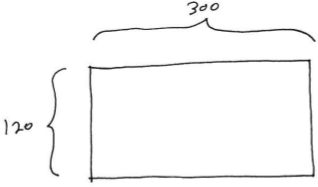
Grid size
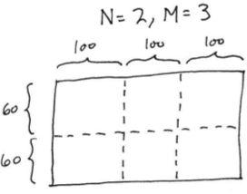
Subdivisions of the grid
The idea is to perform local computation on each process, then communicate them by having process exchange of values who have cells in common. Once the communication is done then perform the next cell generation. The implementation can be more efficient by avoiding the loop over each cell in the grid and sending the values individually to send them all at once but this is a matter for future exploration.
Regarding the feature of rotating the canvas, although I didn’t manage to research it further, I read about some caveats to implement it. I found a thesis about it called Rotations in 2D and 3D discrete spaces by Yohan Thibault and he explains the constraints and challenges that it might face the process of rotating. The loss of precision, lack of neighbor connectivity and artifact appearance are between the common ones. However I’m planning to give it a try and depending on the complexity I may constrain the rotation with 90 degrees steps, and not the total degree freedom as was originally proposed.
Milestone 5 (8 May)
- Implement the canvas rotation
- Implement random map generation
Improve and measure the performance
For this milestone, the goal was to implement the proposed feature of canvas rotation. Initially the conceived idea was to give the user the freedom to rotate the canvas in any angle. As the research went through, the solution seemed not quite trivial and, as mentioned before, a thesis I found detailed the major challenges to tackle this task. In a nutshell, their main problem with making rotations in 2D discrete spaces is the loss of definition as it is shown in the figure below. This happens because the grid to be rotated does not follow the rules of an Euclidean space. To this end the author also proposes a solution using hingle angles which is mutating the matrix with a function of error minimization.

Cumulative pixel lost on canvas rotation
After trying to make a naive implementation on the current simulation, I noticed that there is not so much value to give this feature if the resolution is so low. And considering that the performance is not quite good on high resolution at the moment, an implementation of the rotation was made following the constraints of 90 degrees of freedom. This means that the user can rotate the canvas either clockwise and counterclockwise by one complete rotation at time. To make this possible, a series of transformations over the matrix buffer was required. Rotation by 90 degrees requires to transpose and then reverse each row. Rotation by -90 degrees requires to transpose and then reverse each column.

90 degrees matrix rotation
As a general rule for keeping the properties of the water simulation, only static objects are the ones who can rotate, meaning only blocks who do not interact with gravity.

Constrained canvas rotation
As a bonus feature, I wanted to make a procedural map generation for the water to flow as a quick to-go. For this, a cave map generator based on cellular automata was implemented. This generator returns us a two-dimensional array of blocks, each of which is either solid or empty. So in a sense it resembles a scene of games like dungeon-crawlers with random levels for strategy games and simulation.

Iterative process of CA cave generation
To this end, the procedure is iterative. First we start out by randomly setting each cell to either block or empty. Each cell will have the same random chance of being made alive, 45% in this case. Then after counting the neighbors of each cell we’re going to proceed with the rules of the CA. We have two special variables, one for birthing dead cells (birthLimit), and one for killing live cells (deathLimit). If living cells are surrounded by less than deathLimit cells they die, and if dead cells are near at least birthLimit cells they become alive. Then it’s a matter of try how many iterations this cave generation will take place. The more iterations, the more smoothness can be achieved.

Procedural block generation taking interaction with the fluids
Now speaking of performance improvements. I have been implementing two methods concisely. Parallel processing and compute shaders. I didn’t achieve any positive results from the first method. It required further tweaks and definitely the time to be spended increased a lot. For that reason I decided to give a try to compute shaders. At first I tried to implement the basic Game of Life and the results were quite compelling. The port was relatively easy to do. However when I faced the task of porting the fluid simulation in the shader’s paradigm I encountered many challenges on the way that at the end resulted in me having to look more in depth. Mainly, the problem was that I needed to set up a pipeline of computed processes. The first one for updating the mass value of the cells, and the second pipeline for applying the values of the first buffer into the second by updating the corresponding element type. Since it was the first time doing this it consumed a lot of time and I decided to postpone it for the next and last milestone along with the performance metrics using the criterion library with the test cases that are going to be evaluated.
Milestone 6 (22 May)
- Improve and measure the performance
- Implement extra material(s)
The last milestone of this project was devoted to implementing a bonus element; but first and foremost, to measure and improve the performance of the simulation. To this extent, a GPU version of the simulation was created from scratch, using OpenGL, GLSL and Rust because trying to port the current code to work with shaders was more of a hassle since the library didn’t allow for setup a more complex pipeline rendering. This process involved porting the main computation of the cells into computer shaders.
Benchmark
The benchmarking was done in one computer with three different map setups and two different approaches of rendering: GPU and CPU. The technical specification of the machine is as follows: CPU: Intel i7-7500U @ 3.500GHz 4 cores, RAM: 8GB, GPU: Intel HD Graphics 620. The testbed consisted of three scenarios with different grid sizes to perform the simulation: 250, 500 and 1300 respectively. On each of those, the captured metrics were FPS and time to compute a single simulation step. The resulting average FPS gathered during the evaluation of the three scenarios are shown in the figure below.
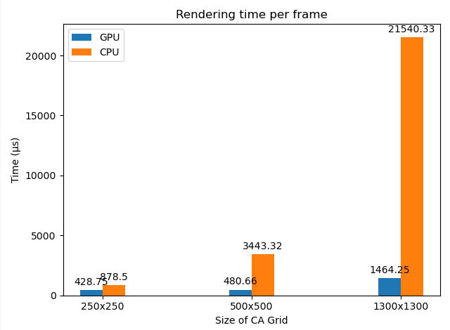
Plot of the time to compute each generation
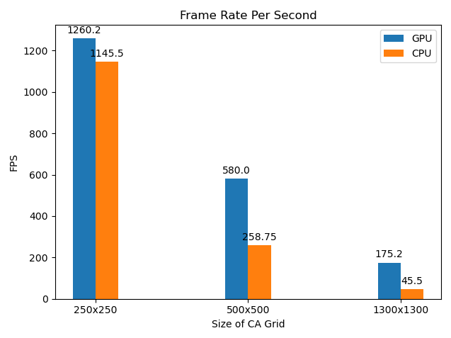
Plot of FPS mean during the simulation
In addition to the CPU version of the CA, the GPU version underlines the effect of parallelization on computation time. It is not surprising that the simulation runs faster on the GPU, but it is still interesting to see the difference in performance. In the figure, with a small grid size the performance is very similar, but as long as the grid size increases we observe that the GPU version is not only much faster than the CPU version but it also scales better. The computation time on the GPU is so small that it scarcely affects the framerate. With this in mind we can say that the computation costs depend on the size of the CA. The size, in turn, depends on the number of cells as well as the number of different elements and is limited by RAM (CPU) and VRAM (GPU).
Bonus element
Since the GLSL version of the code gave room for more graphics experimentation, first the styling was improved, a brush cursor with custom size was introduced, and the new element was well. The extra element is the “acid” or “virus” which behaves by destructing every other “ground” cell that is on its way. It reacts with gravity and it does not last for long.
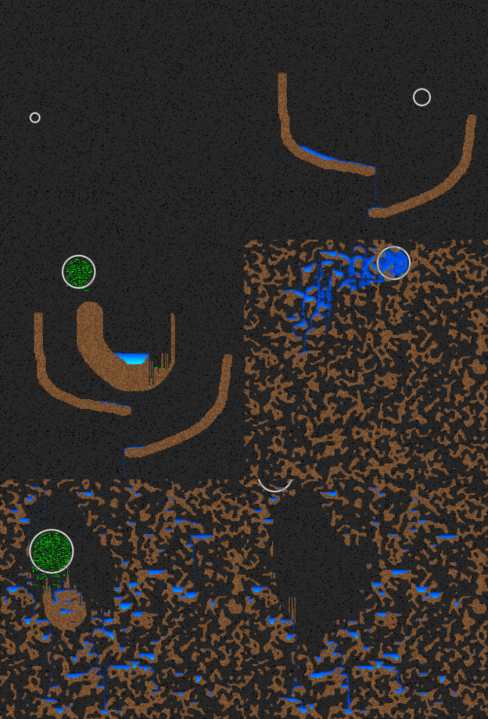
Revamped GPU based simulation
As a conclusion of this milestone I can say that keeping a good performance with an increased grid size was at first a challenge because there were many techniques to approach for dealing with the optimization, however the simplest and cleanest in my opinion was the use of the GPU for computing the simulation, this allowed not only write a cleaner code but also to take advantage and apply more complex shading.
Conclusion
This kind of simulation based on cellular automata, and grid evolution requires a high iteration rate on each frame. By increasing the grid size to make the simulation more realistic comes at the expense of more CPU cycles per frame, making the experience unpleasant. A GPU implementation of the simulation was done to aliviate this. The whole code of the rules was ported to compute shaders and the benchmark shows a dominant increase in performance. I think that was one of the rewarding experiences of this project. I want to thank my classmates and Raimond for the advice and support.
